Compaction
What is Compaction?
When performing inference with a language model, eventually the context length will become too large, resulting in slower and more expensive decoding, along with potentially degraded performance (Hong et al. 2025). Applications such as Claude Code and Codex handle this issue by offering the user a “compaction” feature, which compresses the input tokens into a smaller, more manageable set via summarization.
However, as I’m sure we’ve all seen by interacting with these tools, compaction via summarization can be incredibly lossy, causing model performance to tank. I often find myself scoping sessions to tasks that I know can be reasonably accomplished within a model’s effective context window and using /clear excessively rather than using /compact.
Fast KV Compaction via Attention Matching
To circumvent the issues that come with compacting in token space, researchers have also tried compacting in latent space. Fast KV Compaction via Attention Matching (Zweiger et al. 2026) is a recent paper that poses compaction as a couple of least squares optimization problems.
The problem statement is as follows. At some long sequence length $T$, the model has a KV cache represented by $K,V\in\R^{T\times d}$. The goal is to produce a smaller set of keys and values $C_k,C_v\in\R^{t\times d}$, where $t < T$. Of course, we want to pick this smaller set such that the behavior of the model on the smaller set approximates the behavior of the model on the full set. In the Attention Matching paper, the authors define “behavior” from the perspective of a query vector $q\in\R^{1\times d}$; the attention output and the attention mass of $q$ against the compacted cache should equal the output/mass of $q$ against the full cache. Formally, we want (omitting $\sqrt{d}$ for brevity):
$$ \frac{\exp(qK^\top)V}{\sum_{j=1}^{T}\exp(qK_j^\top)} \approx \frac{\exp(qC_k^\top + \beta)V_k}{\sum_{j=1}^{t}\exp(q(C_k)_j^\top + \beta_j)} $$$$ \sum_{j=1}^{T}\exp(qK_j^\top) \approx \sum_{j=1}^{t}\exp(q(C_k)_j^\top + \beta_j) $$The first equation matches attention output, the second matches attention mass. Matching mass is important when we consider what should happen after compaction: the model needs to attend to the compacted cache plus any new entries to the KV cache. In this case, attention mass determines how much attention probability the compacted cache receives relative to new entries. So, we are essentially “matching the uncompacted cache’s influence during future decoding”.
We include a $\beta$ term because without it, it’s actually impossible to exactly match attention mass due to the compacted cache having a shorter effective sequence length (consider what happens when $q = 0$).
So how do we actually compute $C_k$, $\beta$, and $C_v$? We can do the following:
- Pick $C_k$ by selecting the keys with the highest attention from a set of queries
- Fit $\beta$ using the attention mass equation via NNLS
- Fit $C_v$ using the attention output equation via OLS
Note that we restrict $C_k$ to be a subset of $K$, but there is no such restriction on $C_v$.
The Problem with Attention Matching
Compaction is typically an ad-hoc job. Once we use up too much of the context window in Claude Code, we accept some downtime while running /compact. Faster compaction does have merits though, not just in terms of how users interact with coding agents but also with agents themselves. Autonomous agents that can compact quickly and accurately can complete tasks much more quickly.
The issue with attention matching as proposed above is that although it is much faster than gradient-based methods (Eyuboglu et al. 2025), it can still be quite slow. In order to get a system of equations for fitting $\beta$ and $C_v$, we need multiple queries, each of which will yield one constraint. Ideally, we pick a set of queries that represent the kinds of queries we will see in the future. The most naive choice (and the one we will be using) is “context-prefill”: take the context we’re trying to compact, run it through the model again, and extract all the queries.
Context-prefill results in $Q,K\in\R^{T\times d}$. To compute targets for our NNLS/OLS setup, we will need to perform $QK^\top$, which is quadratic in $T$. Given that we are compacting a long context, $T$ is quite large so needing to perform this matrix multiplication is quite slow. The central question, then, is:
Can we avoid doing $QK^\top$ and instead find a clever way around this massive matmul?
Speeding up Attention Matching by Avoiding $QK^\top$
A simple strategy to doing “approximate attention matching” without $QK^\top$ is as follows:
- Choose $C_k$ without doing $QK^\top$ in such a way that the chosen keys roughly match what would have been chosen if we did the full matmul
- Fit $\beta$
- Fit $C_v$
The hope is that if we pick $C_k$ close enough to what computing full attention would pick and our optimization problems for $\beta$ and $C_v$ are not underdetermined, then we can recover the optimal solution fairly well. Going forward we measure our approximation $C_k$ of $(C_k)\_{\text{full}}$ by measuring overlap: $\frac{|(C_k)\_{\text{full}} \cap C_k|}{t}$. An exact match would have an overlap of 1.0.
Choosing $C_k$
Attempt #1: Expected Attention
The immediate idea that comes to mind is Expected Attention (Devoto et al. 2025). This paper proposes that hidden states (and in turn query vectors, which are just linear transformations of hidden states) loosely follow a multivariate Gaussian distribution. So, instead of computing scores between every query and every key, we can instead just compute scores between a mean query $\bar{q}$ and every key and select $C_k$ based on that.
While being very fast, Expected Attention comes with a few problems that make it difficult to use here:
1. Key selection is NOT similar to full attention
Expected attention despite giving a speed up of ~30x, only has a key selection overlap with full attention of 0.25. It selects very different keys, which means that expected attention does not serve as a good approximator for full attention in this case.
2. Systems for fitting $\beta$ and $C_v$ are very underdetermined
With $T$ queries, we used to have $T$ constraints for fitting $t$ or $t\times d$ unknowns. If we collapse down to just the mean, we end up only have a single constraint each for $\beta$ and $C_v$, resulting in severely underdetermined systems. We can try to fix this by adding ridge regularization or producing more constraints but in practice these work poorly.
3. Queries for Qwen3-4B don’t even follow a Gaussian!
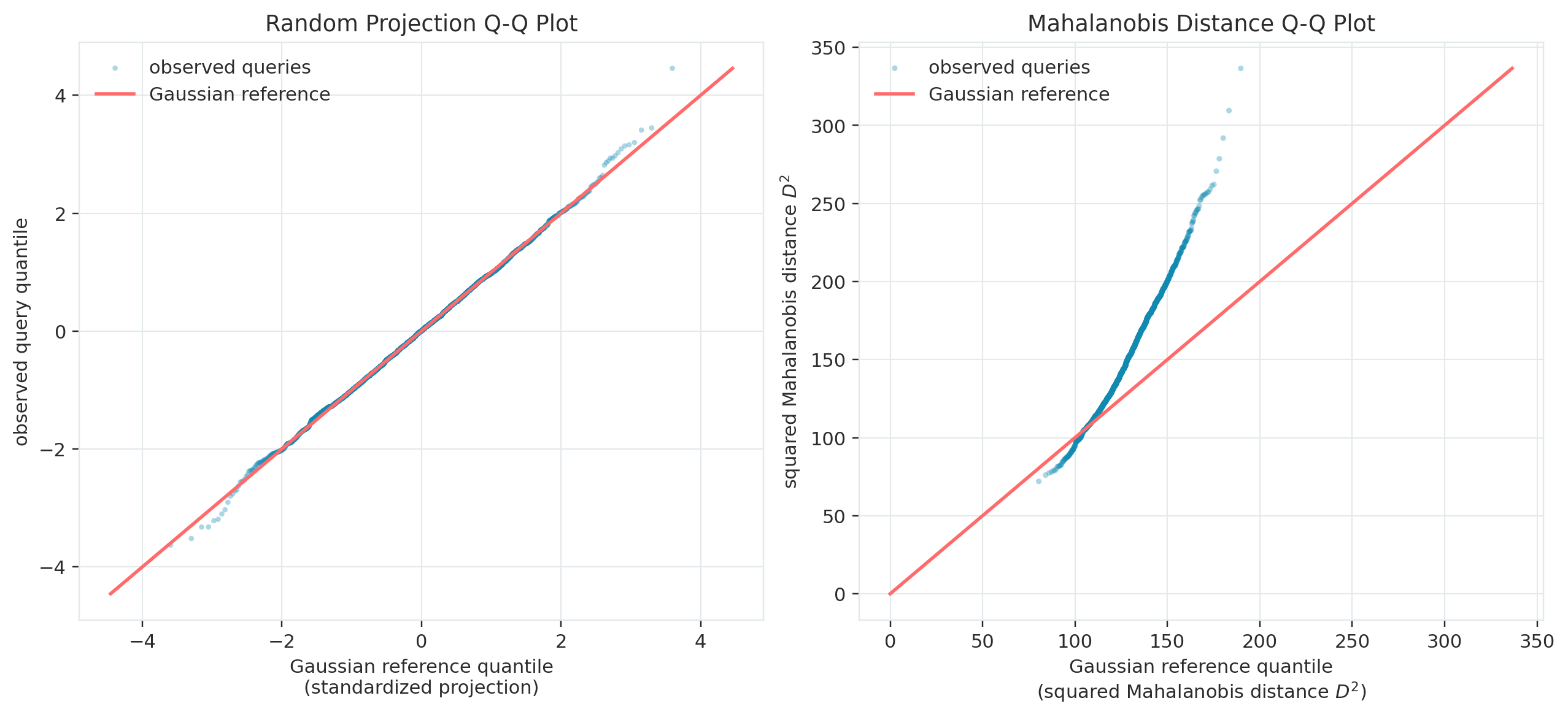
As it turns out, the underlying assumption that the query vectors follow a multivariate Gaussian is wrong! While random 1D projections of the queries are Gaussian, the full query vectors themselves are not. This means that trying to use expected attention for key selection will work quite poorly because we end up missing rare but important query directions.
Attempt #2: Query Subset
Expected attention failed because queries aren’t Gaussian, and also because we lose far too much information collapsing down to just a single average query vector. The next best thing to try is to see if we can optimally pick a small subset of the original queries $Q^\prime$ such that the scores produced by $Q^\prime K^\top$ closely approximate $QK^\top$. This $Q^\prime$ can then be passed on down to fitting $\beta$/$C_v$ as additional constraints, making those systems better determined.
Here are a few different approaches for selecting such queries:
- Random: take a random subset of the original queries
- Mahalanobis: fit a Gaussian on the queries, then select the queries that are the furthest away by Mahalanobis distance
- Principal Components (PC Extreme): fit a Gaussian, do an eigendecomposition on the covariance, then pick the most extreme queries in the positive/negative directions for each principal component of the covariance
The overlap for each method is shown below:
| Method | Overlap with Full Attention |
|---|---|
| Random | 0.43 |
| Mahalanobis | 0.36 |
| PC Extreme | 0.4 |
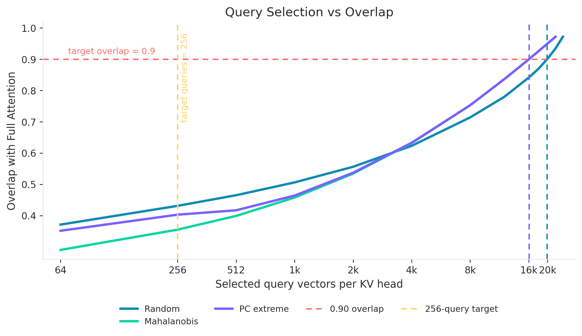
So overlap across these methods is still quite low. Ideally we’d get to ~90% overlap, and then the subsequent fitting steps would just fall into place easily. However, from the figure below, we can see that all three methods are quite inefficient. Getting to 90% overlap requires ~16k-20k queries! There are only ~25k queries total per head/layer, so we’re approaching $O(T)$ queries which defeats any speedup we’re trying to get. Ideally we only need a small fraction of queries (we choose 256 arbitrarily) such that it’s effectively $O(1)$ and we can see an enormous speedup.
Attempt #3: Two-Pass
The prior two attempts make it clear that just finding a subset of queries and computing attention scores with all of the keys is subpar. We can see two main reasons for this by looking at the data from these key selection schemes.
First, consider a key that is chosen by full attention but dropped by one of our selection methods. The top 1% of queries by attention mass contribution have a mean Mahalanobis percentile of 0.53, which essentially means they are NOT outliers. Our Mahalanobis/PC Extreme methods explicitly select outliers, which causes them to miss these critical queries.
Second, for a given key selected by full attention, consider the distribution of how much each query contributes to its overall score. As it turns out, only 0.26% of queries are needed on average to get 50% of a key’s evidence! This explains why just randomly sampling 256 queries misses them: we need a small number of non-outlier queries, and grabbing 256 random ones is simply not precise enough.
So what does it take to get a key selection scheme that is both good and fast? Let’s look at our random sampling method again. We know that it’s far too noisy to select the final set of keys. But what if instead it could give us a shortlist that contains many of the right keys?
To get our final list of $t$ keys, we can sample our random query subset $Q^\prime$ and then compute $Q^\prime K^\top$ to get scores for all $T$ keys. We can choose a subset $kt$ of these keys $K^\prime$, and then do $QK^{\prime\top}$ to get the scores for final key selection.
How big do we need our shortlist to be? The table below shows $k$ versus recall in terms of recovering full attention’s selected keys. At $k=5$ (keeping $5t$ keys as a shortlist), we get a recall of $\approx 0.75$, which is great!
| $k$ | Key Selection Recall |
|---|---|
| 3 | 0.641 |
| 4 | 0.700 |
| 5 | 0.747 |
This two-pass approach gives us huge gains in terms of full attention key overlap:
| Method | Overlap | Speedup Over Full Attention |
|---|---|---|
| Random, 256 queries | 0.431 | 36x |
| Two-Pass, $k=3$ | 0.797 | 3.1x |
| Two-Pass, $k=4$ | 0.852 | 2.4x |
| Two-Pass, $k=5$ | 0.890 | 1.9x |
The tradeoff of course is that Two-Pass is an order of magnitude slower than Random. But we still get a 2x speedup over full attention and we can keep key overlap high.
Choosing $\beta$
Now that we have chosen $C_k$, it’s time to fit $\beta$. As mentioned previously, the way the original Attention Matching paper does this is by solving a non-negative least squares system using the attention mass constraints. To recap, here’s the attention mass matching equation:
$$ \forall q\in Q: \sum_{j=1}^{T}\exp(qK_j^\top) \approx \sum_{j=1}^{t}\exp(q(C_k)_j^\top + \beta_j) $$Note that on the LHS, we still need to compute $QK^\top$ to get a constraint for each query. This is what we wanted to avoid, so we need a workaround. An easy one is to only fit on the queries from $Q^\prime$, the subset of queries we used for key selection. This gives us 256 constraints, and with $t$ unknowns the system can be well determined depending on the compaction ratio.
In practice though, fitting $\beta$ on just 256 random queries works poorly (as we’ll see below). A neat workaround that works surprisingly well is redistribution: distribute the missing mass uniformly among the compacted keys. Formally, for selected key $j$, its unnormalized attention mass over the training queries is:
$$ m_j = \frac{1}{n}\sum_{i=1}^{n}\exp(q_i (C_k)_j^\top) $$The average missing mass from all the dropped keys is the difference between total mass and unbiased compacted mass:
$$ \Delta = \frac{1}{n}\sum_{i=1}^{n}[\sum_{j=1}^{kt}\exp(q_iK_j^{\prime\top}) - \sum_{j=1}^{t}\exp(q_i(C_k)_j^\top)]$$Note that we only consider the shortlist of $kt$ keys $K^\prime$. The purpose of $\beta$ is to distribute $\Delta$ among the chosen keys. Rather than fitting, we just assign $\frac{\Delta}{t}$ to each key, meaning that in the end key $j$ should get mass $m_j + \frac{\Delta}{t}$. This means $\beta_j = \log\frac{m_j + \Delta/t}{m_j}$.
Redistribution is extremely cheap in terms of computation. We already compute $QK^{\prime\top}$ when building $C_k$, which gives us the total mass. The unbiased compacted mass can be derived from $QK^{\prime\top}$ as well because $C_k$ is just a subset of $K^\prime$. So redistribution is essentially free, and gives us huge speedups compared to fitting $\beta$ via NNLS.
But how does it fare in terms of quality? For that, we will look at the mass reconstruction error (how far from the original KV cache’s attention mass the compacted cache + $\beta$ is) on a held-out set of queries:
Here is a table showing mass reconstruction error and wall clock time for each method on three QuALITY articles:
| $\beta$ method | Held-out Error | Wall Clock Time (per head) | Speedup |
|---|---|---|---|
| NNLS | 0.611 | 3.321 ms | 1x |
| Uniform Redistribution | 0.386 | 0.087 ms | 38.4x |
With uniform redistribution, we get a 38.4x speedup while also having a lower error on held-out queries! This is because the queries do not provide enough independent information for NNLS to reliably estimate a separate correction for each key in the compacted cache. In our experiment, we try to fit hundreds of $\beta$ coefficients, but the median effective rank of the NNLS design matrix is ~95, which means that there are many possible $\beta$ that can fit to the training queries ~equally well. Uniform redistribution, on the other hand, introduces a strong inductive bias of no flexibility per-key in exchange for less variance which results in better generalization on unseen queries.
Choosing $C_v$
With $C_k$ and $\beta$ out of the way, we can finally compute the values for our compacted cache. The original Attention Matching paper fits $C_v$ via OLS on attention outputs:
$$ \frac{\exp(qK^\top)V}{\sum_{j=1}^{T}\exp(qK_j^\top)} \approx \frac{\exp(qC_k^\top + \beta)V_k}{\sum_{j=1}^{t}\exp(q(C_k)_j^\top + \beta_j)} $$Once again, we would need to compute $QK^\top$ in order to build the system for OLS to solve. The same issue of an underdetermined system applies if we try to just use $Q'K^\top$ for fitting instead.
This problem is actually really tricky. I tried several approaches to making the optimization problem for $C_v$ better determined:
- adding ridge regularization
- sampling even more queries
- doing a first-order Taylor expansion around the mean query to get more constraints to fit on
and yet all of these did not yield the performance I was looking for. What ended up being the breakthrough was actually thinking about the data and taking a step backwards.
For the purposes of this blogpost, we’re specifically interested in QA tasks (in our case, the QuALITY dataset). We can split the query vectors produced by the model into two groups: the first consists of the queries from the article itself (via context-prefill), and the second consists of the queries from the question asked about the article’s contents (we’ll call these QA queries). The first group is what’s used to produce the compacted cache, while the second group actually uses it. These two groups of queries generally have different attention patterns. context-prefill queries spread their attention across many article tokens, while the QA queries often concentrate attention on a small number of tokens that are relevant to the question being asked.
Now, as a reminder, when we choose to fit $C_v$, the values in the compacted cache are not required to be the same as their corresponding values in the full cache. The compacted values will absorb information from evicted tokens so that the overall attention output remains roughly the same. While this is good for minimizing average attention output error, it can be problematic if a QA query strongly attends to one key. What actually works better in this scenario is retaining the original value vector (we’ll call this approach “direct”). This ensures that the key that the QA query was looking so hard to find has exactly the value that the query was expecting.
The figure below demonstrates this. We take real attention heads from QuALITY and compute how concentrated their attention is on the compacted cache. Then we split the queries up into 4 quartiles based on this concentration (1 being the least concentrated, 4 being the most) and measure the mean error between the original attention output and compacted cache attention output, for both fitted $C_v$ and direct $C_v$. As we can see, directly using $C_v$ matches fitting $C_v$ in terms of reconstructing attention output when attention patterns are diffuse. But as attention gets more concentrated, direct actually ends up beating out fitting.
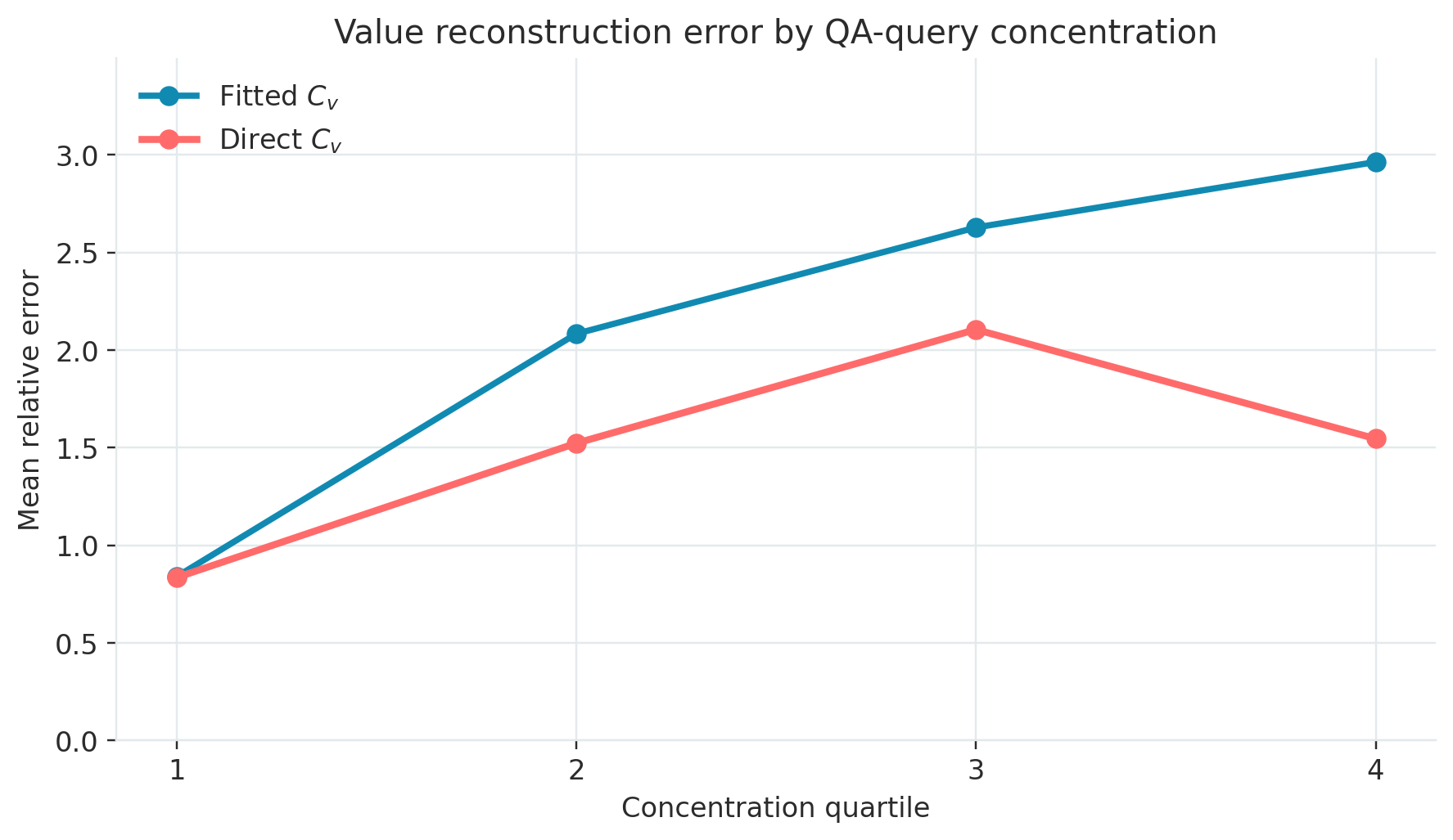
This gives us a reasonable empirical justification for avoiding fitting $C_v$ entirely and using original $C_v$ values instead. This will allow us to speed up compaction time even further, while also potentially improving downstream accuracy. The table below shows detailed numbers on the held-out error/speedup for $C_v$ methods:
| $C_v$ method | Held-out Error | Wall Clock Time (per head) | Speedup |
|---|---|---|---|
| LSQ fitting | 2.128 | 3.044 ms | 1x |
| Direct selection | 1.502 | 0.028 ms | 109.2x |
We can get a lower attention output reconstruction error on held-out queries while also getting a 100x speedup!
Results
While we’ve shown via various proxy metrics (key selection overlap, mean attention mass/output error, etc.) that we can improve compaction quality while reducing wall clock time, the real metric that matters is downstream QA accuracy after KV compaction.
Setup
We evaluate Qwen3-4B on the QuALITY dataset at 5 different compaction ratios: 1%, 2%, 5%, 10%, and 20%. We specifically look at a few different compaction methods to ablate specific techniques:
high_attn: select keys based on highest attention scores via full attention, fit $\beta$ and $C_v$- this is the baseline method proposed by the Attention Matching paper
high_attn_direct: select keys based on highest attention scores via full attention, fit $\beta$, directly use corresponding values to selected keys- tests whether fitting values is necessary for QA tasks
high_attn_redist_direct: select keys based on highest attention scores via full attention, set $\beta$ by uniformly redistributing attention mass, directly use original values- tests whether redistributing $\beta$ is an effective substitute for fitting it
two_pass: select keys using the two-pass approach described previously, set $\beta$ via redistribution, directly use original values- tests whether two-pass key selection is a good approximation for full attention key selection
QuALITY Performance
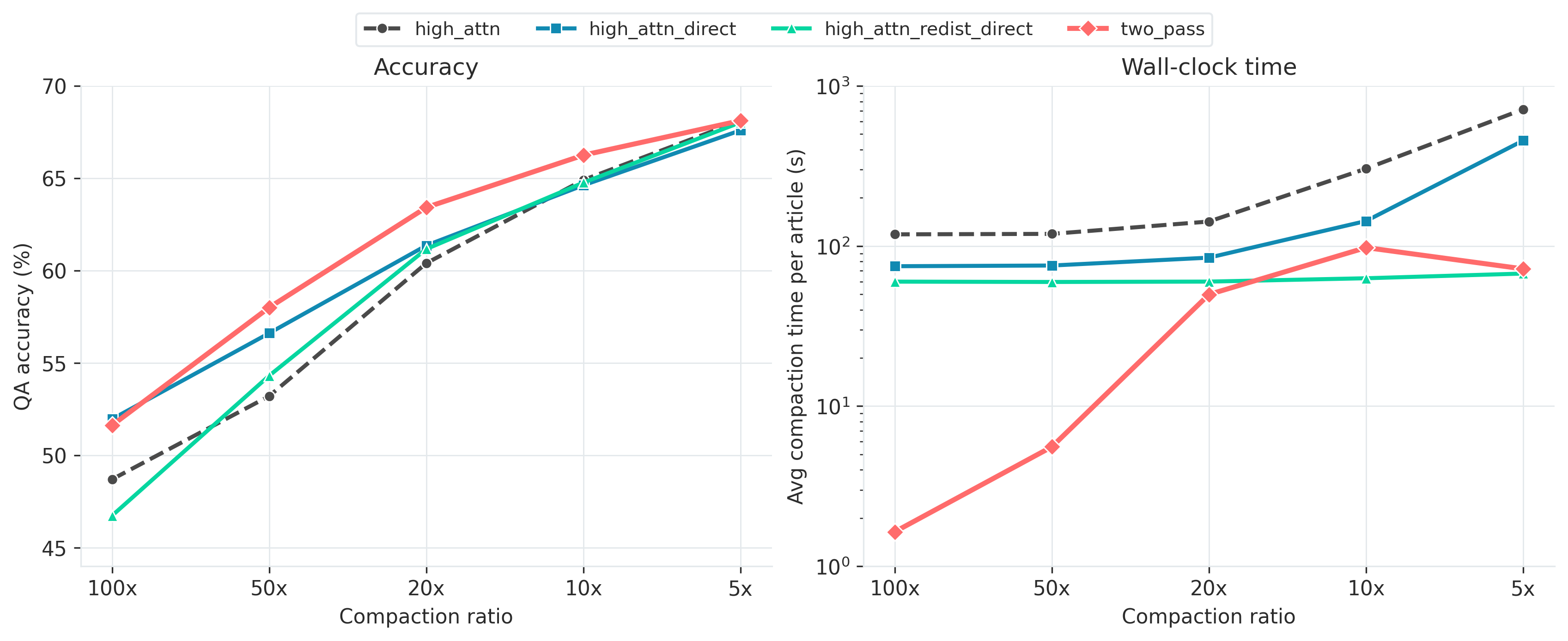
two_pass is much faster than high_attn at any given compaction ratio, for an average speedup of ~6x!
The figure above shows two plots, accuracy on QuALITY and average compaction time per article, for each compaction method and ratio. We follow the same ratios used in the original attention matching paper.
In terms of accuracy, two_pass performs very strongly, beating out high_attn at every compaction ratio except 5x (which is where all methods converge to roughly the same accuracy anyways). At 100x compaction, there’s nearly a ten point gap between the best and worth methods, but this gap shrinks as the compaction ratio decreases. The main takeaway here is that our optimizations do not sacrifice performance and can hold their own against high_attn.
The real impact of our optimizations is visible in the plot for compaction time on the right. high_attn is extremely slow, starting at ~118s per article at 100x compaction and going up to ~714s per article at 5x compaction (the higher time is due to performing least squares on larger systems to fit $\beta$ and $C_v$). That is also why compaction time for high_attn_redist_direct stays flat across ratios: there’s no fitting, so compaction time is approximately just however long it takes to do key selection.
Compaction time increases as compaction ratio decreases for two_pass because as the ratio gets smaller, the number of keys selected gets larger. Remember, if we need $t$ keys, we compute attention on $kt$ keys, with $k$ being some small constant. So compaction time for two_pass does depend on how small we’re compacting to. Regardless, two_pass is much faster than high_attn. At 100x compaction, it has a speed up of two orders of magnitude! And at their closest, two_pass still has a ~6x speedup.
Why does this work?
It’s a bit surprising that two_pass has a better performance than high_attn here, considering it was meant to just be a fast approximation.
Let’s consider the original attention matching problem: we choose a compacted cache with a bias to optimize reconstructed attention on queries using the context-prefill method. Fitting the values of the KV cache using OLS is really good at this and we can reconstruct attention better than if we were to just use the original values directly.
However, as noted previously, the context-prefill queries follow a specific pattern. They typically spread attention broadly across the article while queries that come from the question the model needs to answer exhibit sharp attention patterns. These are the queries that matter to model accuracy and the context-prefill approach to creating reference queries does not incorporate them at all.
There’s another benefit to using values directly. Recall that for QA tasks, attention patterns are more spiky, with only a few entries in the KV cache being strongly attended to. Intuitively, this means that the model really wants the original value at that key. However, if we fit the values instead, that original value changes to fit the overall objective. The model no longer has access to the value it really wanted for that question.
Limitations
While two_pass was quite impressive in the regime of this experiment, I would not expect it to be free lunch everywhere. The fact that QuALITY is a QA benchmark helps our case a lot, as it rewards keeping original values. It’s possible that for summarization/broad reconstruction tasks, fitting the values would work better.
There are some experimental limitations as well. Due to limited compute, I could only use context-prefill to generate reference queries. There are other approaches mentioned in the Attention Matching paper (e.g. repeat-prefill, which essentially repeats the context twice, and self-study, proposed in Cartridges (Eyuboglu et al. 2025), which prompts an LLM for a wide variety of interactions with the context). self-study is expensive, but it performed the best in Attention Matching experiments. The queries that it produces behave similarly to the ones from downstream tasks (e.g. sharp attention patterns for QA), which makes it a good objective to fit on.
Conclusion
The main takeaway from these experiments is that if you want good, fast compaction for QA tasks, you don’t need to do full attention reconstruction. In the context of QA tasks, the goal of KV compaction is slightly different. The model should keep the right keys/values for later retrieval when answering a question.
So, we make a few tweaks:
- swapping full $QK^\top$ attention computation for a cheaper, two-pass approach
- redistribute missing mass into a bias term $\beta$, rather than fitting it via NNLS
- use original values directly rather than fitting them to prioritize keeping relevant facts in the KV cache
The result is a compaction method that is up to two orders of magnitude faster, while maintaining performance on the original attention matching baseline!